Author: Jordan Watson (jordan.watson@noaa.gov) and Matt Callahan (mcallahan@psmfc.org)

Apologies for the temporary disruption in service - the web API is being replaced with a newer and more functional version. The data are also being transitioned to a longer time series (from MUR SST to Coral Reef Watch SST). We’re also working on integrating some marine heatwave functionality. It’ll be worth it! You can see some interim developments with the new web API here (https://github.com/jordanwatson/AKFIN_WebService). Meanwhile, updated SST and marine heatwave plots can be generated here: https://mattcallahan.shinyapps.io/NBS_SEBS_SST_MHW/

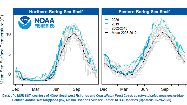
The data are downloaded daily through the NOAA CoastWatch West Coast Node ERDDAP, and ingested at AKFIN, the Alaska Fisheries Information Network. For each day, approximately 10 million temperature records are aggregated into the Alaska Department of Fish and Game statistical management areas. Within each of these areas and on each day, the data are averaged to yield 1,758 daily average SST records (one sst record per stat area). These data are then binned into regional spatial strata as described by the NOAA Alaska Fisheries Science Center Ecosystem Status Consideration spatial strata, “Eastern Bering Sea (EBS)”, “Northern Bering Sea (NBS)”, “Western Gulf of Alaska (WGOA)”, and the “Eastern Gulf of Alaska (EGOA)”. These daily regional SST values are available via a public webAPI at AKFIN.

The aksst package can be installed for R from github.

library(devtools)
install_github("jordanwatson/aksst")

Currently there are only a few basic functions. The data are updated daily and the full time series is updated when running the update_sst_data() function. A message will notify users that this may take 10-20 seconds to download the data.

library(aksst)
sstdata <- update_sst_data()

There are four regions that can be easily examined, “EBS”, “NBS”, “EGOA”, “WGOA”. The scaling works best if Bering Sea plots are kept together and GOA plots are kept together. Current formatting is for two areas at a time. A future version may include a single area.

A single function will output a formatted png file to the working directory, with the NOAA logo and some metadata at the bottom.

Assuming you read in the data above, you could generate images with the following:

#  Using the sstdata object created above, plot the data
plot_ak_sst(sstdata,"EBS","NBS")
plot_ak_sst(sstdata,"EGOA","WGOA")

To plot a generic version to your R console, you can use the generic plotting function that omits the NOAA logo and metadata.

plot_ak_sst_generic(sstdata,"EBS","NBS")
plot_ak_sst_generic(sstdata,"WGOA","WGOA")

If you knew you just wanted to plot a single image, then there’s no need to save the data as a separate object and you could just use the integrated update and plot function in a single step.

update_and_plot_ak_sst("EBS","NBS")

This is the same thing as just updating within the first argument.

plot_ak_sst(update_sst_data(),"EBS","NBS")

For more information on the spatial strata, see descriptions in the Bering Sea and Gulf of Alaska Ecosystem Status Reports (keyword search for Watson).

For more information about methods, see this contribution in the Pacific States e-Journal for Scientific Visualizations.

Package developed and maintained by Jordan Watson. Comments and thoughts are my own and do not represent NOAA or the National Marine Fisheries Service.